The “Practical-Graphical-Analytical” strategy enhancing our data analyses

How to apply the "P.G.A." approach and two classic examples on how to take advantage of this, although the authors of the examples didn't mention that.

“Ars est celaree artem” - Ovidio (art to conceal art)

Abstract:

• The Practical-Graphical-Analytical method is summarized and two classic examples are described to illustrate how it improves data analyses;

• Confusion of correlation and causation example from Box and Hunter [2] was used to present what can happen when Practical part of P.G.A. is neglected;

• The “Boys Shoes” example from the same reference was used to illustrate a complete P.G.A. approach.

According to dictionary.com, the quote above means “true art conceals the means by which it is achieved”. This can happen by chance in improvement projects, if you automatically use a method, not necessarily realizing that. That was not the case of the cited authors of the examples brought to this text but could be the case of many project leaders that apply the approach to be illustrated and may not have even been aware they were doing so.

The “P.G.A.” approach consists of three fundamental dimensions when we analyze data. When we apply such a strategy, we are disciplining ourselves in merging our specific knowledge and the improvement science that, only together, lead us to actual improvements. I couldn’t find the author of this method but, since I learned that during a Black Belt training in 2007, I have found it extremely useful in every improvement or innovation project. You can also use this in any data interpretation process [1] and reduce the risk of misinterpretations.

The first, is based on our experience in the specific area we intend to improve. For example, I could develop a process improvement in any area. Let's say sales, which is not my expertise, but if I get the right people involved, which have this know-how and, sum up this with the Lean Six Sigma Methodology (the science of improvement), we can together develop improvements in the commercial area.

The Practical approach would deal with observing actual data (i.e. large enough differences, trends, patterns, unusual observations..). We can understand this additionally as bringing our know-how into this improvement process plus the raw data gathering and analysis (what were we expecting, if data makes sense, if we can trust the measuring system, if we can translate them into something meaningful for us..) . When we are measuring our process on site, we can take notes of the overall process, unexpected happenings, and practical observations we may have during this collection. If we are familiar with the phenomenon being analyzed or just aware because we have been trained (e.g. a Lean Six Sigma Belt looking for wastes) we get critical information by thoroughly observing the events.

The graphical approach is brought when we translate data into a visual summary such as a histogram, a dot plot or a Control Chart. Such illustration can carry several crucial findings, besides a much easier understanding of data location (most expected values, as means or medians), variation (how much the data is spread) and shape (how exactly is the distribution form). Through graph analysis we can better understand how our data is distributed in regards to these features.

Analytical approach means performing statistical analyses such as hypothesis tests, calculating statistics that add objectivity to our studies as descriptive statistics or employing tools such as Design of Experiments, Correlation and Regression Analyses, etc.

Although some of us might assume that one of these approaches can solely suffice, after some years of project management in improvement endeavors, we all understand that we must bring all these views into discussion before making any conclusion. Let’s illustrate this with two classic statistics examples..

The Storks of Oldenburg

At Box and Hunter [2] you can find several examples of how one can use statistics to reach good conclusions. On page 8 though, they exemplify from another reference data [3] how experimenters can make confusions between correlation and causation. You can also find several examples on the internet of such confusions. (Picture from Alexas_Fotos by Pixabay)

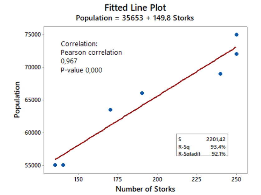
In this case, data were collected correlating a small German city population and the number of storks there. Some people could hypothesize, from the results, that the increase of population could be caused by the increase of storks number. This hypothesis could be handy whenever we need to explain to our children where babies come from. The authors argue that this could be explained by a correlation of both variables with a third factor (e.g. time). This could also be the case that storks number increase would be caused by population increase (more chimneys to serve as nest places).

Remembering the Practical approach is bringing our experience to support the analysis, we realize this is necessary for a proper conclusion. Either Graphical (as the extract below adapted from Box and Hunter [1]) or Analytical approach (e.g. by calculating the strong correlation factor) could lead us to a wrong conclusion.

The Boys’ Shoes Experiment

Box and Hunter [2] had also presented an interesting example of how the strategy behind the experiment may help us achieve more realistic results. Again, they didn’t explicitly mention a "P.G.A." approach but it can be understood as a good example of one of those.

(Picture from Free-Photos by Pixabay)

The goal was to analyze the performance of two materials regarding wear. Some of us could easily consider a group with material “A” and another group with the cheaper material “B”. This type of experiment would bring together variation we wouldn’t want to measure such as the intensity of each boy's activities, weight, the conditions of pavement they walk on, and several other aspects not interesting to our experiment together with the wear change between materials.

The experiment was then run in pairs. Each boy wore a pair of shoes with both materials. Therefore, the variation we could not control was reduced while the change of our interest, to mention, the difference between the materials could be better analyzed.

The data collected is summarized below, where (L) means that the material was used for the left foot shoe and (R) used for the other side shoe. The decision of which boy would use a specific material in each foot was randomized.

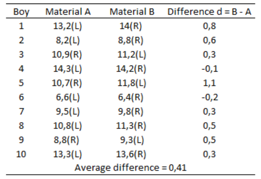
The Practical approach in this case is illustrated by our knowledge of the phenomenon, for example: what we know about wear. We might have not taken in consideration, as the authors did, the fact that this feature is much more impacted by the differences among the boys, that we can’t control, than the differences of the materials. We can notice that by looking over the raw data. Therefore, if we hadn’t planned these experiments in pairs, we would probably not find any difference between the materials. WIth experiment made in pairs, we notice that only with two boys, the difference was negative, i.e. the wear was higher for Material A. So we have first signal that this material is better for this feature.

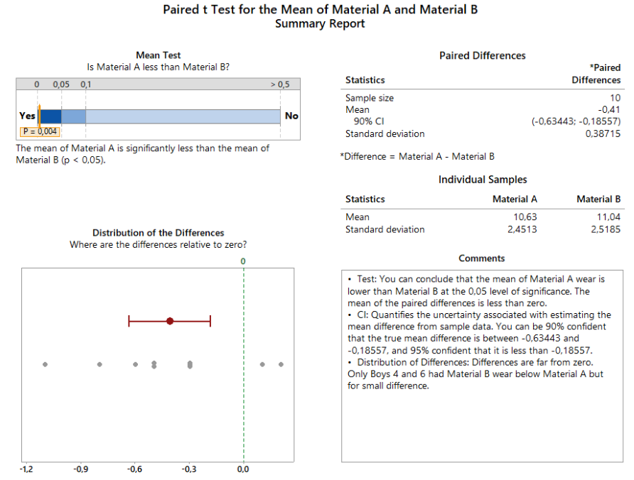
For a Graphical analysis, we could plot either individual values or the differences as below. It already gives the same conclusion, which is: Material B presents a higher wear.

Finally, the analytical approach could be illustrated with a hypothesis test. You can find below the summary of the paired t test performed in Minitab. Data were previously tested for normal distribution fit.

Conclusion

The “P.G.A.” strategy helps us to bring our expertise into data analysis. All three approaches must be held in order to reduce the risk of biased conclusions.

Sometimes the statistics may be planned or analyzed in a distorted way due to our lack of knowledge about ƒthe phenomenon being studied. In these cases, bringing together different views over the same data can help us identify unusual results and eventually review our experimentation plan.

References

[1] http://www.leanmath.com/blog-entry/pga-t-meaningfully-interpret-data-four-steps

[2] Box, E.P., Hunter J.S. and Hunter W.G., Statistics for Experimenters: Design, Innovation, and Discovery, Wiley Series in Probability and Statistics

[3] Fisher, G., Ornithologische Monatsberichte, 44, no. 2, Jahrgang, 1936 and 38 no. 1, Jahrgang, 1940, Berlin and Statistisches, Jahrbuch Deutscher Gemeinden, 27-22, Jahrgang, 1932-1938